Depth: Analysis of the core technology behind the automatic driving of Tesla
Speaking of Tesla, you may immediately think of a life-threatening accident in the Tesla Model S driverless in May this year. Preliminary investigations revealed that under strong daylight conditions, both the driver and the driverless system failed to notice the white body of the towed trailer, so the brake system could not be activated in time. And because the towed trailer is crossing the road and the body is high, this special situation causes the Model S to collide with the bottom of the trailer when it passes through the bottom of the trailer, causing the driver to die.
Coincidentally, on August 8, Joshua Neally, a man from Missouri, USA, and Tesla Model X owner, burst into a pulmonary embolism on his way to work. With the help of Model X's Autopilot driverless function, he arrived safely at the hospital. This "one by one and one promotion" is really memorable, and it means that "there is also a defeat, Xiao He, and Cheng Xiaohe".

Curious readers must have doubts: What is the principle behind this "one-on-one failure"? Which part of the driverless system has a mistake and caused a car accident? Which part of the technology supports the driverless process?
Today, let's talk about an important core technology in the driverless system - semanTIc image segmentaTIon. Image semantic segmentation is an important part of image understanding in computer vision. Not only is the demand in the industry increasingly prominent, but semantic segmentation is also one of the research hotspots in the current academic world.
What is image semantic segmentation?Image semantic segmentation can be said to be the cornerstone technology of image understanding, which plays an important role in unmanned systems (specifically streetscape recognition and understanding), drone applications (landing point judgment) and wearable device applications.
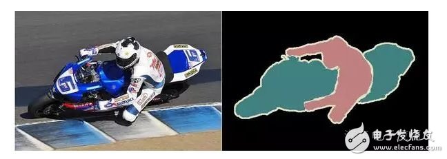
We all know that an image is composed of many pixels, and "semantic segmentation", as its name implies, groups (grouping)/segmentation of pixels according to the semantic meaning of the expression in the image. The figure below is taken from one of the standard data sets in the field of image segmentation, PASCAL VOC. The left picture is the original image, and the right picture is the ground truth of the segmentation task: the red area represents the image pixel area with the semantics "person", the blue-green represents the "motorbike" semantic area, the black represents the "background", white (Edge) indicates an unmarked area.
Obviously, in the image semantic segmentation task, the input is a H × W × 3 three-channel color image, and the output is a corresponding H × W matrix. Each element of the matrix indicates the corresponding position pixel in the original image. The semantic label of the representation. Therefore, image semantic segmentation is also referred to as "image semantic labeling", "semantic pixel labeling" or "semantic pixel grouping".
From the above figure and the title map, it can be clearly seen that the difficulty of the image semantic segmentation task lies in the word "semantic". In real images, the same object that expresses a certain semantic is often composed of different parts (eg, building, motorbike, person, etc.), and these parts often have different colors, textures, and even brightness (such as building), which gives image semantics. Accurate segmentation presents difficulties and challenges.
Semantic segmentation in the pre-DL eraFrom the simplest pixel-level "thresholding methods", clustering-based segmentation methods, to graph partitioning segmentation methods, deep learning (deep learning) , DL) Before the "unification of the rivers and lakes", the work of image semantic segmentation can be described as "a hundred flowers bloom." Here, we only use the two methods of normal segmentation based on "normalized cut" [1] and "grab cut" [2] as an example to introduce the research on semantic segmentation in the pre-DL era.
The Normalized cut (N-cut) method is one of the most famous methods of semantic partitioning based on graph partitioning. In 2000, Jianbo Shi and Jitendra Malik published in the related field TPAMI. In general, the traditional semantic segmentation method based on graph partitioning abstracts the image into a graph of the form G=(V, E) (V is the graph node, E is the edge of the graph), and then uses graph theory. The theory and algorithm in the image segmentation of the image.
A common method is the classic min-cut algorithm. However, the classic min-cut algorithm only considers local information when calculating the weight of the edge. As shown in the figure below, taking the bipartite graph as an example (dividing G into disjoint, two parts), if only local information is considered, then separating a point is obviously a min-cut, so the result of the graph division is similar or This is out of the group, and from a global perspective, the group that actually wants to divide is the left and right.
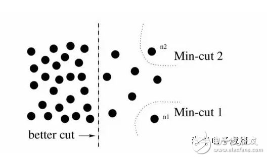
In response to this situation, N-cut proposes a method of considering global information for graph partitioning, that is, the weight of the connection between the two partitions A, B and the full graph node (assoc (A, V) and assoc(B,V)) are taken into account:
In this way, in the outlier division, one of the items will be close to 1, and such a picture division obviously cannot make it a small value, so the purpose of considering the global information and discarding the separation group point is abandoned. Such an operation is similar to the normalization operation of features in machine learning, so it is called normalized cut. N-cut can not only handle two types of semantic segmentation, but also expand the bipartite graph into K-way (-way) graph partitioning to complete multi-semantic image semantic segmentation, as shown in the following illustration.
Grab cut is a well-known interactive image semantic segmentation method proposed by Microsoft Cambridge Research Institute in 2004. Like N-cut, the grab cut is also based on graph partitioning, but the grab cut is an improved version that can be thought of as an iterative semantic segmentation algorithm. Grab cut takes advantage of texture (color) information and boundary (contrast) information in the image, so that a small amount of user interaction can get better background segmentation results.
In the grab cut, the foreground and background of the RGB image are modeled using a Gaussian mixture model (GMM). Two GMMs are used to characterize the probability that a pixel belongs to the foreground or background, and the number of each GMM gaussian component is generally set.
Next, the gibbs energy function is used to globally characterize the whole image, and then iteratively finds the parameters that make the energy equation reach the optimal value as the optimal parameters of the two GMMs. Once the GMM is determined, the probability that a pixel belongs to the foreground or background is determined.
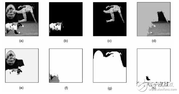
In the process of interacting with the user, the grab cut provides two ways of interaction: one with a bounding box as the auxiliary information and the other with a scribbled line as the auxiliary information. In the following figure, for example, the user provides a bounding box at the beginning. Grab cuts the default to think that the pixel in the box contains the main object/foreground. After that, it is solved by iterative graph division, and then the foreground result is returned. It can be found even for With a slightly more complex background image, the grab cut still performs well.

However, the segmentation effect of the grab cut is unsatisfactory when processing the image below. At this point, additional artificial information is needed to provide additional auxiliary information: the background area is marked with red lines/dots, and the foreground area is indicated by white lines. On this basis, run the grab cut algorithm again to obtain the optimal solution to get a satisfactory semantic segmentation result. Grab cut Although the effect is excellent, but the shortcomings are also very obvious, one can only deal with the second type of semantic segmentation problem, and the second is the need for human intervention and can not be fully automated.

In fact, it is not difficult to see that the semantic segmentation work in the pre-DL era is based on the low-level visual cues of the image pixels themselves. Since such a method does not have an algorithm training phase, the computational complexity is often not high, but on a more difficult segmentation task (if no artificial auxiliary information is provided), the segmentation effect is not satisfactory.
After computer vision enters the era of deep learning, semantic segmentation has also entered a new stage of development, with a series of convolutional neural networks "training" represented by fully convolutional networks (FCN). Methods have been proposed successively, and the accuracy of image semantic segmentation is frequently updated. The following describes three representative practices in the field of semantic segmentation in the DL era.
Full convolutional neural network
The full convolutional neural network FCN is arguably the groundbreaking work of deep learning on image semantic segmentation tasks. It was published by UC Berkeley's Trevor Darrell group and was published in CVPR 2015, the top conference in computer vision, and won the best paper honorable mention.
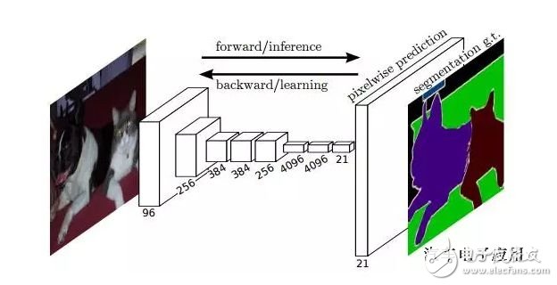
The FCN's idea is straightforward, that is, direct pixel-level end-to-end semantic segmentation, which can be implemented based on the mainstream deep convolutional neural network model (CNN). In the so-called "full-convolution neural network", in the FCN, the traditional fully-connected layers fc6 and fc7 are implemented by the convolutional layer, and the final fc8 layer is replaced by a 21-channel 1x1 convolutional layer. As the final output of the network. There are 21 channels because the PASCAL VOC contains 21 categories (20 object categories and one "background" category).
The following figure shows the network structure of the FCN. If the original picture is H×W×3, the response tensor corresponding to the original picture can be obtained after several stacking convolution and pooling operations, where is the i-th layer. The number of channels. It can be found that due to the downsampling effect of the pooling layer, the length and width of the response tensor are much smaller than the length and width of the original image, which brings problems to the direct training at the pixel level.
In order to solve the problem caused by downsampling, FCN uses bilinear interpolation to upsample the length and width of the response to the original image size. In addition, in order to better predict the details in the image, the FCN also responds to the shallow layer in the network. Also consider coming in. Specifically, the responses of Pool4 and Pool3 are also taken as the outputs of the models FCN-16s and FCN-8s, respectively, combined with the output of the original FCN-32s for the final semantic segmentation prediction (as shown below). .

The following figure shows the semantic segmentation results of different layers as outputs. It can be clearly seen that different semantic segmentation levels are caused by the different downsampling ratios of the pooling layer. For example, FCN-32s, because it is the convolution and pooling output of the last layer of FCN, the model has the highest downsampling multiple, and the corresponding semantic segmentation result is the coarsest; while FCN-8s can be obtained because the downsampling factor is small. More detailed segmentation results.

Dilated Convolutions
One disadvantage of FCN is that the size of the response tensor (length and width) is getting smaller and smaller due to the presence of the pooling layer, but the original design of the FCN requires an output that is consistent with the input size, so the FCN is upsampled. . However, upsampling does not completely retrieve the lost information.
In this regard, dilated convolution is a good solution - since the pooled downsampling operation will bring information loss, then the pooling layer is removed. However, the removal of the pooling layer brings down the receptive field of each layer of the network, which reduces the prediction accuracy of the entire model. The main contribution of Dilated convolution is how to remove the pooled downsampling operation without reducing the network's receptive field.
Taking a 3×3 convolution kernel as an example, when performing a convolution operation, the traditional convolution kernel multiplies the convolution kernel by the “continuous†3×3 patch in the input tensor and then sums it (see the following figure a). The red dot is the input "pixel" corresponding to the convolution kernel, and the green is its perception field in the original input). The convolution kernel in the classified convolution is a convolution operation of a 3 × 3 patch of input tensors separated by a certain number of pixels.
As shown in the following figure b, after removing the layered layer, the traditional convolution layer needs to be replaced by a "dilation=2" dilated convolution layer after the removed pooling layer. At this time, the convolution kernel will input the tensor. Every other "pixel" position is used as the input patch for convolution calculation. It can be found that the perception field corresponding to the original input has been dilated. Similarly, if a pooling layer is removed, it will be followed. The convolutional layer is replaced by the classified convolution layer of "dilation=4", as shown in Figure c. In this way, even if the pooling layer is removed, the network's receptive field can be guaranteed, thereby ensuring the accuracy of image semantic segmentation.

It can be seen from the following image semantic segmentation renderings that the use of the dilated convolution technique can greatly improve the recognition of semantic categories and the fineness of segmentation details.

Post-processing operation represented by conditional random field
The current image semantic segmentation based on deep learning uses the conditional random field (CRF) as the final post-processing operation to optimize the semantic prediction results.
In general, CRF treats the category to which each pixel in the image belongs as a variable, and then considers the relationship between any two variables to create a complete graph (as shown in the following figure).
In a fully linked CRF model, the corresponding energy function is:

Where is a unary item representing the semantic category corresponding to the pixel, the category of which can be obtained from the prediction of the FCN or other semantic segmentation model; and the second term is a binary term, which can consider the semantic association/relationship between pixels Go in. For example, the probability that pixels such as "sky" and "bird" are adjacent in physical space should be greater than the probability of adjacent pixels such as "sky" and "fish". Finally, by optimizing the CRF energy function, the image semantic prediction results of FCN are optimized, and the final semantic segmentation result is obtained.
It is worth mentioning that there is already work [5] to embed the CRF process originally isolated from the deep model training into the neural network, that is, to integrate the FCN+CRF process into an end-to-end system. The energy function that is the final prediction result of CRF can be directly used to guide the training of FCN model parameters, and obtain better image semantic segmentation results.

Outlook
As the saying goes, "no free lunch". The image semantic segmentation technology based on deep learning can achieve the segmentation effect compared with the traditional method, but its requirements for data annotation are too high: not only need massive image data, but also need to provide accurate pixel-level markup information ( Semantic labels). As a result, more and more researchers are turning their attention to the problem of image semantic segmentation under weakly-supervised conditions. In such problems, images only need to provide image-level annotation (for example, "people", "car", no "television") without the need for expensive pixel-level information to achieve semantic segmentation comparable to existing methods. Precision.
In addition, the image level segmentation problem of the instance level is also popular. This kind of problem not only requires image segmentation for different semantic objects, but also requires segmentation of different individuals of the same semantics (for example, the pixels of the nine chairs appearing in the figure need to be marked with different colors).

Finally, video-based video segmentation is one of the new hotspots in the field of computer visual semantic segmentation. This setting is more suitable for the real application environment of driverless systems.
According to: Wei Xiuxin, the author of this article, Xie Chenwei, Department of Computer Learning and Data Mining (LAMDA), Department of Computer Science, Nanjing University, research direction for computer vision and machine learning.
References:
[1] Jianbo Shi and Jitendra Malik. Normalized Cuts and Image Segmentation, IEEE Transactions on Pattern Analysis and Machine Intelligence, Vol. 22, No. 8, 2000.
[2] Carsten Rother, Vladimir Kolmogorov and Andrew Blake. "GrabCut"--Interactive Foreground Extraction using Iterated Graph Cuts, ACM Transactions on Graphics, 2004.
[3] Jonathan Long, Evan Shelhamer and Trevor Darrell. Fully Convolutional Networks for Semantic Segmentation. IEEE Conference on Computer Vision and Pattern Recognition, 2015.
[4] Fisher Yu and Vladlen Koltun. Multi-scale Context Aggregation by Dilated Convolutions. International Conference on Representation Learning, 2016.
[5] Shuai Zheng, Sadeep Jayasumana, Bernardino Romera-Paredes, Vibhav Vineet, Zhizhong Su, Dalong Du, Chang Huang and Philip HS Torr. Conditional Random Fields as Recurrent Neural Networks. International Conference on Computer Vision, 2015.
SCOTECH offers a full range of special transformers for both AC and DC voltages. Including AC/DC Furnace Transformer , Rectifier Transformer, Grounding Transformer, K Rated Transformer, traction transformer, and other special application transformers, with years of experience, lots references from different applications and a global operation footprint, SCOTECH is experienced to make the customer's special application transformer.
By using the best quality of materials for the transformer core and windings, a reduction of losses has been achieved. For the end-user this means that with lower losses, more economy, and makes the payback time of the investment shorter. The lifetime of the transformer is also extended.
Why SCOTECH
Long history- Focus on transformer manufacturing since 1934.
Technical support – 134 engineers stand by for you 24/7.
Manufacturing-advanced production and testing equipment, strict QA system.
Perfect service-The complete customer service package (from quotation to energization)
Special Transformer,Earthing Transformer,Traction Transformer,Phase Shifting Transformer
Jiangshan Scotech Electrical Co.,Ltd , https://www.scotech.com