Comparison of TPA and RRA (case analysis)

The most common methods of negative feedback circuit analysis are dual port analysis (TPA) and regression ratio (RRA) analysis. The two are different and similar, and often confusing. This design example uses two familiar circuit examples to illustrate these two techniques. In the two block diagrams of Figure 1, the subscripts TP and RR are used to distinguish between the two types of dual port and regression ratio.

Specifically, αTP and αRR are open loop gains, and ßTP and ßRR are feedback coefficients. Figure 1a is assumed to be a unidirectional block, and Figure 1b is more versatile because it also takes into account the feedthrough around the error amplifier, as indicated by the gain block αft.

Figure 1: (a) A negative feedback block diagram of the dual port (TP) and (b) regression ratio (RR) analysis.

Depending on whether sI and sO are voltage or current, there are four possible topologies, as shown in the op amp of Figure 2. In each of the sub-graphs, the front of the hyphen refers to the way the input is added (series voltage, parallel current), and the one after the hyphen refers to the way the feedback network samples sO to generate the feedback signal sF ( Parallel voltage, series current). For each topology, the closed-loop gain is presented as:

among them:

It is the loop gain, and Aideal is the value of sO/sI in the limit condition (TTP → ∞), which is obtained by making αTP → ∞. In addition, the feedback factor is:

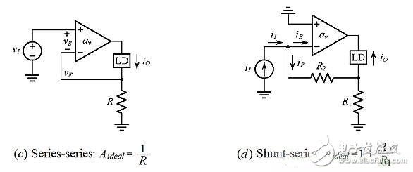
Figure 2: Using an op amp to illustrate four basic feedback topologies.

TPA seeks an alphaTP expression that takes into account any interaction (such as loading) between the amplifier and the feedback network. Negative feedback converts the open-loop resistance of each port, rpa, into a closed-loop resistor, making this task easy:

It is +1 in the case of series and -1 in the case of parallel. If the TTP is large enough, R can be considered as an open circuit in the case of a series connection and as a short circuit in the case of a parallel connection.

As a first example, we apply TPA to the current amplifier of Figure 3a, which has:

To get αTP, we modified the error amplifier as shown in Figure 3b. The resistance seen by the input source in Figure 3a is Ri = R2 / (1 + αv), and the resistance seen by the load is Ro = R1 (1 + αv). For large αv, we expect Ri to be small and Ro to be large. Therefore, if we approximate Ro as an open circuit (OC), the feedback network seen from the input port of the amplifier is a simple series combination of R2 + R1. Again, if we

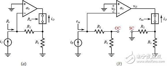
Figure 3: (a) Parallel-series configuration terminated with short-circuit load; (b) Circuit using TPA to find open-loop parameters αTP, ria, and roa.

Comparing Ri to short circuit (SC), the feedback network seen from the amplifier output port is a simple parallel combination of R2//R1. So we have:

Indicates that the open loop gain is:

Note that αTP ≠ αv. Simplified loop gain:

Rethink the example of αv = 10 V/V and R1 = R2 = 10kΩ. Bring the equation above, giving:

Although there are approximations of OC and SC, this is quite advantageous compared to Aexact = 1.909 A/A derived from direct analysis. To ensure that this approximation is not accidental, let's check the values ​​of Ri and Ro. By examining Figure 3b, we have ria = R2 + R1 and roa = R2 / / R1. Using equation (4), we get:

This confirms that Ri is much smaller than the other resistors in the circuit, and Ro is much larger.

This method, as shown in the block diagram of Figure 1b, calculates the closed-loop gain:

Among them, TRR is the loop gain, and Aideal and αft are the values ​​of sO/sI under the conditions of TRR → ∞ and TRR → 0, respectively. These limits are achieved by making αRR → ∞ and αRR → 0 in Figure 1b. According to the following process, the regression ratio of the TRR to the dependent source αRRsE of the error amplifier is obtained:

(a) Set sI → 0; (b) Immediately cut off the feedback loop immediately downstream of the slave source αRRsE; (c) Test signal sT of the same type and polarity as the source of αRRsE passes downstream of the circuit; (d) Found by the slave source itself The returned signal sR; (e) Obtain the loop gain as the regression ratio.

As the analysis progressed, we found that it is convenient to express TRR as a product, similar to equation (2):

Get the feedback coefficient βRR:

Or more simply, βRR = TRR / αRR.

Applying this process to the current amplifier of Figure 3a produces the circuit of Figure 4a. By checking, we have vR = αvvD = αv(–vT), so:

Therefore, αRR = αv and βRR = TRR/αRR = 1. Let αv → 0 to get the feedthrough gain, as shown in Figure 4b. By checking, iO = iI, so αft= iO/iI = 1 A/A. Considering the example of αv = 10V/V and R1= R2 = 10kΩ, we now have:

Comparing equations (14) with (8), observe the difference in values ​​of each of T, α, and β. In addition, ARR is accurate, while ATP is only approximate. In order to comply with the assumption of using a unidirectional block in Figure 1a, the TPA is as close as possible to Aexact by making TTP = 20 (compared to TRR = 10). For the current value of αv, making TTP = 21 (instead of 20) will result in ATP = Aexact, which can be easily verified. However, it does not work for lower values ​​where the feedthrough becomes more relevant (eg, αv = 1V/V). When αv = 0, the difference is the largest, where ARR=Aexact=1 V/V, but ATP = 0.

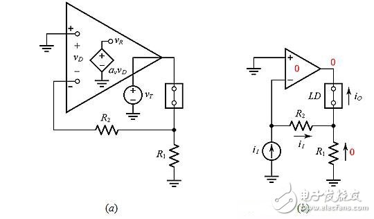
Figure 4: Circuitry for obtaining (a) loop gain TRR and (b) feedthrough gain αft for the current amplifier of Figure 3a.

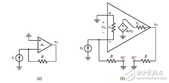
Figure 5: (a) Parallel-parallel configuration; (b) Circuit with error gain αTP.

We apply these two methods to the IV converter of Figure 5a, but use a more realistic op amp model with a non-infinite input impedance ri and a non-zero output impedance ro. As we know, this circuit has:

Since this is a parallel-parallel topology, the feedback resistor is the ground resistance of both the input and output ports, as shown in Figure 5b. We have:

Indicates open loop gain:

Pay attention to αTP ≠αv again. Moreover, the loop gain is:

For RRA, please refer to the circuit of Figure 6, which gives:

So the loop and feedthrough gain is simplified to:

Note that αft and Aideal are opposite in polarity. We compare the two methods for a specific situation that is easy to imagine, namely αv = 60 V/V and ri= ro = R = 10kΩ. Yes, with a less qualified op amp, you can better show the difference. Bring this data into the relevant formula and get:

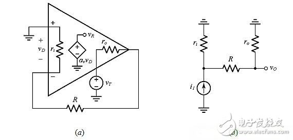
Figure 6: Circuitry for obtaining (a) loop gain TRR and (b) feedthrough gain αft for the IV converter of Figure 5a.

Note the difference in magnitude, polarity and dimension of αTP and αRR and βTP and βRR. There are also subtle differences between ATP and ARR (=Aexact).

If the op amp ro = 0, there will be no feedthrough according to equation (18). In this case, we will get: TTP = TRR = 30, ATP = ARR = –9.677V/mA. If the op amp also has ri = ∞, then TTP = TRR = 60 and ATP = ARR = –9.836 V/mA. However, there will still be large differences, namely αTP = –600 V/mA and βTP = −0.1 mA/V, and αRR = 60 V/V and βRR = 1. Despite the differences, these two parameter sets will still try to provide the same A value!

Two more examples

Finally, let's take a look at the single transistor circuit of Figure 7a and b. The common small-signal model in Figure 7c shows that the error gain is based on gm (in the op amp's box, it is based on αv). Moreover, both circuits are series-input type. However, depending on whether we use the output as the emitter voltage vo or the collector current io, there are parallel-output or series-output types, respectively. Both circuits are simple and can be analyzed directly. However, research through TPA and RRA will be more instructive.

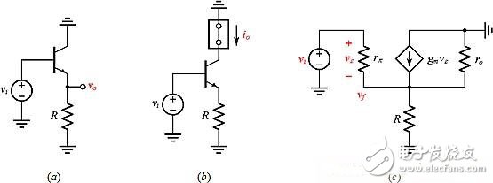
Figure 7: Assume gm = 40mA/V, rπ = 2.5kΩ, ro = 40kΩ and R = 1.0kΩ. (a) series-parallel circuits; (b) series-series circuits; (c) their common small-signal model.

● Figure 7a TPA of the series-parallel circuit: To get Aideal, let gm → ∞, as shown in Figure 8a. This makes vε→ 0 or vo → vi, meaning Aideal = 1.0V/V (= 1/βTP). Referring to Figure 8b, by inspection we have vo = gm(R//ro)vε or αTP=vo/vε=gm(R//ro). Bring in the data, you can get:

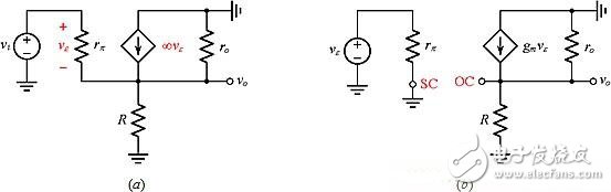
Figure 8: Circuitry for obtaining (a) Aideal and (b) αTP for the series-parallel circuit of Figure 7a.

● Figure 7a RRA of the series-parallel circuit: To get the TRR, see Figure 9a, where ir = gmvπ = gm[(-it)(rπ//R//ro)]; to get αft, see Figure 9b, where vo = vi(R//ro)/[rπ + (R//ro)]. and so:

Bring in the data and get:

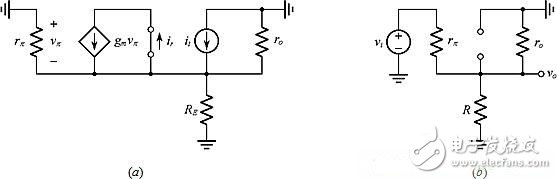
Figure 9: Circuitry for obtaining (a) TRR and (b) alpha ft of the series-parallel circuit of Figure 7a.

● Figure 7b TPA of series-series circuit: To find Aideal, let gm → ∞, as shown in Figure 10a. This causes vε → 0, resulting in a virtual short on rπ, so iR = vi/R. The KCL at the supernode gives io = iR = vi/R, so Aideal=io/vi=1/R(=1/βTP). To get αTP, continue as shown in Figure 10b. The results are as follows:

Bring in the data and get:

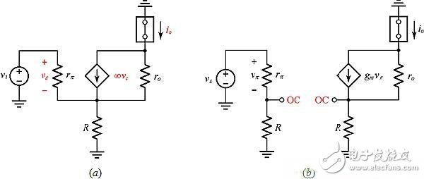
Figure 10: Circuitry for obtaining (a) TRR and (b) alpha ft for the series-series circuit of Figure 7b.

• Figure 7b RRA of the series-series circuit: To derive the TRR, see Figure 11a. This is the same as Figure 9a, so we have the same TRR. To get αft, continue as shown in Figure 11b. The results are as follows:

Bring in the data and get:

The feedthrough of the series-series circuit is smaller than that of the series-parallel circuit, so ATP → ARR.

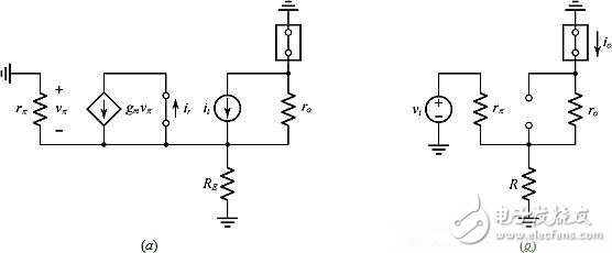
Figure 11: Circuitry for obtaining (a) TRR and (b) αft for the series-series circuit of Figure 7b.

All four feedback topologies are discussed above using a simple circuit with op amps and transistors as gain components (the gain of the op amp is αv and the transistor is gm). Comparing the process and results, we found that:

RRA is more versatile than TPA because it takes into account the feedthrough around the error amplifier. Therefore, the results of the RRA are accurate, and the results of the TPA are only approximate. For high loop gain, the difference between TPA and RRA is minimal, and the difference is greatest when the loop gain drops to zero, where ARR → αft but ATP → 0. TPA calculates the loop gain as the product TTP = αTPβTP; RRA calculates it as the ratio TRR = –vR/vT. TPA uses different dual-port representations for each of the four feedback topologies, so in general, the αTP, βTP, and TTP of different topologies will be different. In contrast, the loop gain TRR for a given circuit is independent of the topology, but depends on the type and location of the input and output signals (but αft is usually related to the topology). Both analyses are handled differently for any interaction between the error amplifier and the feedback network, such as loading. TPA assumes βTP = 1/Aideal and then manipulates the amplifier circuit by using OC and SC approximations to obtain αTP, so usually αTP≠αv (or αTP≠gm). In addition to breaking the signal injection loop, the RRA does not affect the operation of the circuit. RRA assumes αRR = αv (or αRR = gm), which shifts the effects of the interaction between the error amplifier and the feedback network to the feedback network itself, so usually βRR≠1/Aideal. TTP and TRR may sometimes be the same, but this should not be taken as a normal state. In particular, you should not use TRR to calculate ATP, or use TTP to calculate ARR. For example, an error that occurs when trying to use equation (3). RRA feels more intuitive and more suitable for computer simulation or testing in the lab. On the other hand, TPA forces you to parse the circuit in a way that more reveals the interaction between the amplifier and the feedback network.

OVNS Mesh Vape Series

OVNS Mesh Vape Series is so convenient, portable, and small volume, you just need to take them
out of your pocket and take a puff, feel the cloud of smoke, and the fragrance of fruit surrounding you. It's so great.
We are the distributor of the ovns & vapeak vape brand, we sell ovns disposable vape,ovns vape kit, ovns juul compatible refillable pod, and so on.
We are also China's leading manufacturer and supplier of Disposable Vapes puff bars, disposable vape kit, e-cigarette
vape pens, and e-cigarette kit, and we specialize in disposable vapes, e-cigarette vape pens, e-cigarette kits, etc.

ovns mesh vape bar,ovns mesh vape pen,ovns mesh vape starter kit,ovns mesh vape disposable,ovns mesh vape box

Ningbo Autrends International Trade Co.,Ltd. , https://www.ecigarettevapepods.com